Interval Linear Systems

This section provides an overview of functions for obtaining estimates of the solution set for interval linear systems.

First, connect the necessary modules:

>>> import intvalpy as ip
>>> import numpy as np

Solution Variability

def ive(A, b, N=40)

When solving a system, we typically obtain many different estimates, all equally valid as answers to the problem and consistent with the given data. Variability characterizes how small or large this solution set is.

To obtain a quantitative measure, use the ive function:

Parameters:

• AInterval

  The input interval matrix of the interval system of linear algebraic equations (ISLAE), which can be either square or rectangular.

• bInterval

  The interval right-hand side vector of the ISLAE.

• Nint, optional

  The number of corner matrices for which the condition number is calculated. By default, N = 40.

Returns:

• outfloat

  A measure of the variability of an interval system of linear equations, denoted IVE.

Notes:

A randomized algorithm is used to speed up calculations, so there is a chance that a non-optimal value might be found. To mitigate this, you can increase the value of the parameter N.

Examples:

>>> A = ip.Interval([
...     [[98, 100], [99, 101]],
...     [[97, 99], [98, 100]],
...     [[96, 98], [97, 99]]
... ])
>>> b = ip.Interval([[190, 210], [200, 220], [190, 210]])
>>> ip.linear.ive(A, b, N=60)
1.56304

For more information, see the article by S.P. Shary.

The Boundary Intervals Method

When it becomes necessary to visualize the solution set of a system of linear inequalities (or an interval system of equations) and obtain all vertices of the set, one can resort to methods for solving the vertex enumeration problem. However, existing implementations have several drawbacks: they only work with square systems and handle unbounded sets poorly.

Based on the application of the boundary intervals matrix, the boundary intervals method was proposed for studying and visualizing polyhedral sets. The main advantages of this approach are its ability to work with unbounded and thin solution sets, as well as linear systems where the number of equations differs from the number of unknowns.

The main steps of the algorithm are:

1. Formation of the boundary intervals matrix;

2. Modification of the boundary intervals matrix considering the plotting window;

3. Construction of ordered vertices of the polyhedral solution set;

4. Output of the constructed vertices and (if necessary) rendering of the polyhedron.

2D Visualization of a Linear Inequality System

To work with a system of linear algebraic inequalities A x >= b in two unknowns, use the lineqs function. If the solution set is unbounded, the algorithm will automatically choose plotting boundaries. However, the user can specify them explicitly.

Parameters:

• A: float

  The matrix of the system of linear algebraic inequalities.

• b: float

  The right-hand side vector of the system of linear algebraic inequalities.

• show: bool, optional

  If True, the solution set is plotted. Default is True.

• title: str, optional

  The title of the plot.

• color: str, optional

  The fill color for the solution set.

• bounds: array_like, optional

  The boundaries of the plotting window. The first element of the array corresponds to the lower bounds for the OX and OY axes, and the second to the upper bounds. For example, to set OX in the range [-2, 2] and OY in [-3, 4], use bounds=[[-2, -3], [2, 4]].

• alpha: float, optional

  The transparency of the plot.

• s: float, optional

  The size of the vertex points.

• size: tuple, optional

  The size of the plotting window (width, height).

• save: bool, optional

  If True, the plot is saved.

Returns:

• out: list

  A list of ordered vertices. If show=True, the plot is also displayed.

Examples:

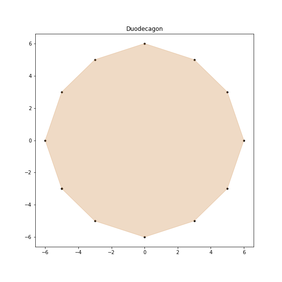
Consider a system describing a dodecagon:

>>> A = -np.array([[-3, -1],
...               [-2, -2],
...               [-1, -3],
...               [1, -3],
...               [2, -2],
...               [3, -1],
...               [3, 1],
...               [2, 2],
...               [1, 3],
...               [-1, 3],
...               [-2, 2],
...               [-3, 1]])
>>> b = -np.array([18,16,18,18,16,18,18,16,18,18,16,18])
>>> vertices = ip.lineqs(A, b, title='Duodecagon', color='peru', alpha=0.3, size=(8,8))
array([[-5., -3.], [-6., -0.], [-5.,  3.], [-3.,  5.], [-0.,  6.], [ 3.,  5.],
       [ 5.,  3.], [ 6.,  0.], [ 5., -3.], [ 3., -5.], [ 0., -6.], [-3., -5.]])

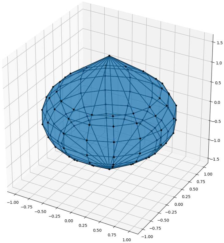
3D Visualization of a Linear Inequality System

To work with a system of linear algebraic inequalities A x >= b in three unknowns, use the lineqs3D function. If the solution set is unbounded, the algorithm will automatically choose plotting boundaries. However, the user can specify them explicitly. To indicate that the solution set is truncated by the plotting window, the clipping planes are colored red.

Parameters:

• A: float

  The matrix of the system of linear algebraic inequalities.

• b: float

  The right-hand side vector of the system of linear algebraic inequalities.

• show: bool, optional

  If True, the solution set is plotted. Default is True.

• color: str, optional

  The fill color for the solution set.

• bounds: array_like, optional

  The boundaries of the plotting window. The first element corresponds to the lower bounds for the OX, OY, and OZ axes, and the second to the upper bounds. For example, to set OX in [-2, 2], OY in [-3, 4], and OZ in [1, 5], use bounds=[[-2, -3, 1], [2, 4, 5]].

• alpha: float, optional

  The transparency of the plot.

• s: float, optional

  The size of the vertex points.

• size: tuple, optional

  The size of the plotting window (width, height).

Returns:

• out: list

  A list of ordered vertices. If show=True, the plot is also displayed.

Examples:

Consider a system describing a «spinning top» (Yula):

>>> %matplotlib notebook
>>> k = 4
>>> A = []
>>> for alpha in np.arange(0, 2*np.pi - 0.0001, np.pi/(2*k)):
...     for beta in np.arange(-np.pi/2, np.pi/2, np.pi/(2*k)):
...         Ai = -np.array([np.sin(alpha), np.cos(alpha), np.sin(beta)])
...         Ai /= np.sqrt(Ai @ Ai)
...         A.append(Ai)
>>> A = np.array(A)
>>> b = -np.ones(A.shape[0])
>>>
>>> vertices = ip.lineqs3D(A, b)

Visualizing the Solution Set of an ISLAE with Two Unknowns

To work with an interval linear system of algebraic equations A x = b in two unknowns, use the IntLinIncR2 function.

To construct the solution set, the main problem is divided into four subproblems. This utilizes the convexity property of the solution within each orthant of R² and the Beeck characterization. This results in systems of linear inequalities in each orthant, which can be visualized using the lineqs function.

If the solution set is unbounded, the algorithm will automatically choose plotting boundaries. However, the user can specify them explicitly.

Parameters:

• AInterval

  The input interval matrix of the ISLAE, which can be square or rectangular.

• bInterval

  The interval right-hand side vector of the ISLAE.

• show: bool, optional

  If True, the solution set is plotted. Default is True.

• title: str, optional

  The title of the plot.

• consistency: str, optional

  Parameter for selecting the type of solution set. If consistency=“uni“, the function returns the united solution set. If consistency=“tol“, it returns the tolerable solution set.

• bounds: array_like, optional

  The boundaries of the plotting window. The first element corresponds to the lower bounds for the OX and OY axes, and the second to the upper bounds. For example, to set OX in [-2, 2] and OY in [-3, 4], use bounds=[[-2, -3], [2, 4]].

• color: str, optional

  The fill color for the solution set.

• alpha: float, optional

  The transparency of the plot.

• s: float, optional

  The size of the vertex points.

• size: tuple, optional

  The size of the plotting window (width, height).

• save: bool, optional

  If True, the plot is saved.

Returns:

• out: list

  Returns a list of ordered vertices in each orthant, starting from the first and moving in a positive direction. If show=True, the plot is also displayed.

Examples:

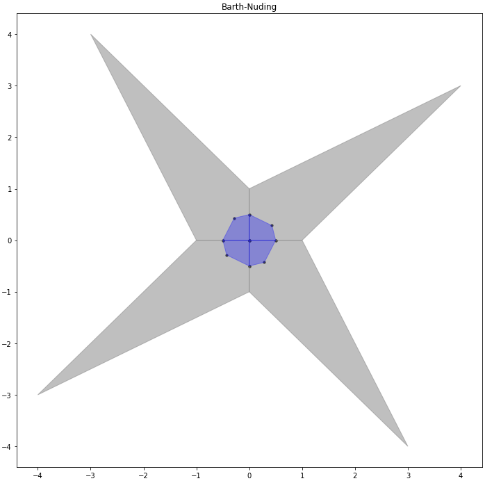
Consider the well-known interval system proposed by Barth-Nuding. To illustrate how different solution types vary, plot the united and tolerable sets on the same graph:

>>> import matplotlib.pyplot as plt
>>>
>>> A = ip.Interval([[2, -2],[-1, 2]], [[4,1],[2,4]])
>>> b = ip.Interval([-2, -2], [2, 2])
>>>
>>> fig = plt.figure(figsize=(12,12))
>>> ax = fig.add_subplot(111, title='Barth-Nuding')
>>>
>>> vertices1 = ip.IntLinIncR2(A, b, show=False)
>>> vertices2 = ip.IntLinIncR2(A, b, consistency='tol', show=False)
>>>
>>> for v in vertices1:
...     if len(v) > 0:  # if intersection with the orthant is not empty
...         x, y = v[:,0], v[:,1]
...         ax.fill(x, y, linestyle='-', linewidth=1, color='gray', alpha=0.5)
...         ax.scatter(x, y, s=0, color='black', alpha=1)
>>>
>>> for v in vertices2:
...     if len(v) > 0:
...         x, y = v[:,0], v[:,1]
...         ax.fill(x, y, linestyle='-', linewidth=1, color='blue', alpha=0.3)
...         ax.scatter(x, y, s=10, color='black', alpha=1)

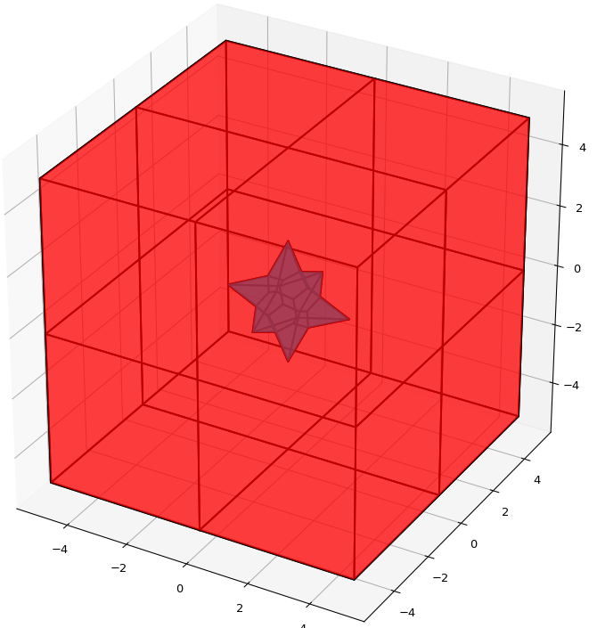
Visualizing the Solution Set of an ISLAE with Three Unknowns

To work with an interval linear system of algebraic equations A x = b in three unknowns, use the IntLinIncR3 function.

To construct the solution set, the main problem is divided into eight subproblems. This utilizes the convexity property of the solution within each orthant of R³ and the Beeck characterization. This results in systems of linear inequalities in each orthant, which can be visualized using the lineqs3D function.

If the solution set is unbounded, the algorithm will automatically choose plotting boundaries. However, the user can specify them explicitly. To indicate that the solution set is truncated by the plotting window, the clipping planes are colored red.

Parameters:

• AInterval

  The input interval matrix of the ISLAE, which can be square or rectangular.

• bInterval

  The interval right-hand side vector of the ISLAE.

• show: bool, optional

  If True, the solution set is plotted. Default is True.

• consistency: str, optional

  Parameter for selecting the type of solution set. If consistency=“uni“, the function returns the united solution set. If consistency=“tol“, it returns the tolerable solution set.

• bounds: array_like, optional

  The boundaries of the plotting window. The first element corresponds to the lower bounds for the OX, OY, and OZ axes, and the second to the upper bounds. For example, to set OX in [-2, 2], OY in [-3, 4], and OZ in [1, 5], use bounds=[[-2, -3, 1], [2, 4, 5]].

• color: str, optional

  The fill color for the solution set.

• alpha: float, optional

  The transparency of the plot.

• s: float, optional

  The size of the vertex points.

• size: tuple, optional

  The size of the plotting window (width, height).

Returns:

• out: list

  Returns a list of ordered vertices in each orthant. If show=True, the plot is also displayed.

Examples:

Consider an interval system where the solution is the entire region except the interior:

>>> %matplotlib notebook
>>> inf = np.array([[-1,-2,-2], [-2,-1,-2], [-2,-2,-1]])
>>> sup = np.array([[1,2,2], [2,1,2], [2,2,1]])
>>> A = ip.Interval(inf, sup)
>>> b = ip.Interval([2,2,2], [2,2,2])
>>>
>>> bounds = [[-5, -5, -5], [5, 5, 5]]
>>> vertices = ip.IntLinIncR3(A, b, alpha=0.5, s=0, bounds=bounds, size=(11,11))

References for the Boundary Intervals Method

[1] I.A. Sharaya - Boundary intervals method for visualization of polyhedral solution sets // Computational Technologies, Vol. 20, No. 1, 2015, pp. 75-103. (In Russian)

[2] P.A. Shcherbina - Boundary intervals method in the free computer mathematics system Scilab (In Russian)

[3] S.P. Shary - Finite-Dimensional Interval Analysis. (In Russian)

Methods for Solving Square Systems

This section presents algorithms for solving square interval systems of equations.

The Gaussian Elimination Method

The Gaussian elimination method, including its various modifications, is an extremely popular algorithm in computational linear algebra. Therefore, its interval version is also available, which consists of two stages — forward elimination and back substitution.

Parameters:

• AInterval

  The input interval matrix of the ISLAE, which must be square.

• bInterval

  The interval right-hand side vector of the ISLAE.

Returns:

• outInterval

  An interval vector that, when substituted into the system of equations and after performing all operations according to the rules of arithmetic and analysis, yields true equalities.

Examples:

Consider the well-known interval system proposed by Barth-Nuding:

>>> A = ip.Interval([[2, -2],[-1, 2]], [[4, 1],[2, 4]])
>>> b = ip.Interval([-2, -2], [2, 2])
>>> ip.linear.Gauss(A, b)
interval(['[-5.0, 5.0]', '[-4.0, 4.0]'])

The Interval Gauss-Seidel Method

def Gauss_Seidel(A, b, x0=None, C=None, tol=1e-12, maxiter=2000)

An iterative method for obtaining outer estimates of the united solution set for an interval system of linear algebraic equations (ISLAE).

Parameters:

• AInterval

  The input interval matrix of the ISLAE, which must be square.

• bInterval

  The interval right-hand side vector of the ISLAE.

• X: Interval, optional

  An initial guess interval vector within which to search for the outer estimate. By default, X is an interval vector with each element set to [-1000, 1000].

• C: np.array or Interval, optional

  A matrix for preconditioning the system. By default, C = inv(mid(A)).

• tol: float, optional

  The tolerance. If the width of an interval falls below this value, it is considered zero for convergence purposes.

• maxiter: int, optional

  The maximum number of iterations.

Returns:

• outInterval

  An interval vector representing an outer estimate of the united solution set.

Examples:

>>> A = ip.Interval([
...     [[2, 4], [-2, 1]],
...     [[-1, 2], [2, 4]]
... ])
>>> b = ip.Interval([[1, 2], [1, 2]])
>>> ip.linear.Gauss_Seidel(A, b)
Interval(['[-10.6623, 12.5714]', '[-11.0649, 12.4286]'])

Preconditioning the system with the inverse of the midpoint matrix can yield a wider outer estimate than if a specially selected preconditioning matrix were used. The system below is the same as above but preconditioned with a specially selected matrix.

>>> A = ip.Interval([[0.5, -0.456], [-0.438, 0.624]],
...                  [[1.176, 0.448], [0.596, 1.36]])
>>> b = ip.Interval([0.316, 0.27], [0.632, 0.624])
>>> ip.linear.Gauss_Seidel(A, b, C=ip.eye(A.shape[0]))
Interval(['[-4.26676, 6.07681]', '[-5.37144, 5.26546]'])

Parameter Partitioning Methods (PPS)

def PPS(A, b, tol=1e-12, maxiter=2000, nu=None)

PPS — optimal (exact) componentwise estimation of the united solution set for an interval linear system of equations.

x = PPS(A, b) computes optimal componentwise lower and upper estimates of the solution set for the interval linear system of equations Ax = b, where A is a square interval matrix and b is an interval right-hand side vector.

x = PPS(A, b, tol, maxiter, nu) computes the vector x of optimal componentwise estimates of the solution set for the interval linear system Ax = b with an accuracy no more than tol and after no more than maxiter iterations. The optional input argument nu specifies the component number of the interval solution for which estimates are to be computed. If this argument is omitted, all componentwise estimates are computed.

Parameters:

• A: Interval

  The input interval matrix of the ISLAE, which can be square or rectangular.

• b: Interval

  The interval right-hand side vector of the ISLAE.

• tol: float, optional

  The tolerance. If the width of an interval falls below this value, it is considered zero for convergence purposes.

• maxiter: int, optional

  The maximum number of iterations.

• nu: int, optional

  The index of the component for which the solution set is evaluated. If None, all components are evaluated.

Returns:

• out: Interval

  An interval vector representing the optimal componentwise estimates.

Examples:

>>> A, b = ip.Neumeier(5, 10)
>>> ip.linear.PPS(A, b)
Interval(['[-0.214286, 0.214286]', '[-0.214286, 0.214286]', '[-0.214286, 0.214286]', '[-0.214286, 0.214286]', '[-0.214286, 0.214286]'])

References for Square System Methods

[1] R.B. Kearfott, C. Hu, M. Novoa III - A review of preconditioners for the interval Gauss-Seidel method // Interval Computations, 1991-1, pp 59-85

[2] S.P. Shary - Finite-Dimensional Interval Analysis.

[3] S.P. Shary, D.Yu. Lyudvin - Testing Implementations of PPS-methods for Interval Linear Systems // Reliable Computing, 2013, Volume 19, pp 176-196

Methods for Solving Overdetermined Systems

When dealing with an overdetermined interval system of linear algebraic equations (ISLAE), simply discarding equations to make the system square can lead to a solution vector that contains an optimal estimate of the solution set. However, this approach can significantly worsen (inflate) the estimate, which is highly undesirable. Therefore, specific algorithms for solving overdetermined systems are needed.

Rohn’s Method

The method proposed by J. Rohn in [1] for obtaining a solution vector is based on solving an auxiliary square linear inequality. This inequality is constructed using the most representative point matrix Ac from the interval matrix A, i.e., Ac = mid(A). The implemented algorithm is a simple variation of the algorithm proposed in the article and does not provide an optimal estimate of the solution set.

Parameters:

• AInterval

  The input interval matrix of the ISLAE, which can be square or rectangular.

• bInterval

  The interval right-hand side vector of the ISLAE.

• tolfloat, optional

  The tolerance. If the width of an interval falls below this value, it is considered zero for convergence purposes.

• maxiterint, optional

  The maximum number of iterations for the algorithm.

Returns:

• outInterval

  An interval vector representing an estimate of the solution set.

Examples:

Consider the well-known interval system proposed by Barth-Nuding:

>>> A = ip.Interval([[2, -2],[-1, 2]], [[4,1],[2,4]])
>>> b = ip.Interval([-2, -2], [2, 2])
>>> ip.linear.Rohn(A, b)
Interval(['[-14, 14]', '[-14, 14]'])

This example demonstrates that the solution can be far from optimal, which in this case is Interval([„[-4, 4]“, „[-4, 4]“]).

As a second example, consider the test system by S.P. Shary:

>>> A, b = ip.Shary(4)
>>> ip.linear.Rohn(A, b)
Interval(['[-4.34783, 4.34783]', '[-4.34783, 4.34783]', '[-4.34783, 4.34783]', '[-4.34783, 4.34783]'])

Unlike the previous example, this solution vector is quite close to the optimal outer estimate.

Solution Splitting Method (PSS)

A hybrid method for solution splitting, known as PSS, described in detail in [2]. PSS algorithms are designed to find optimal outer estimates of the solution sets for interval systems of linear algebraic equations (ISLAE) A x = b.

As the basic method for outer estimation, the interval Gaussian method (function Gauss) is used if the system is square. If the system is overdetermined, the simple algorithm proposed by J. Rohn (function Rohn) is applied. Since the problem is NP-hard, the process may stop based on the number of iterations completed. PSS methods are sequentially guaranteeing, meaning that if the process is terminated after any number of iterations, the approximate solution estimate still satisfies the required estimation criterion.

It returns a formal solution of the interval linear system of equations. If it is not necessary to estimate all components, any single nu-th component can be estimated.

Parameters:

• AInterval

  The input interval matrix of the ISLAE, which can be square or rectangular.

• bInterval

  The interval right-hand side vector of the ISLAE.

• tolfloat, optional

  The tolerance. If the width of an interval falls below this value, it is considered zero for convergence purposes.

• maxiterint, optional

  The maximum number of iterations for the algorithm.

• nuint, optional

  The index of the component along which the solution set is estimated. If None, all components are estimated.

Returns:

• outInterval

  An interval vector representing the estimate of the solution set.

Examples:

>>> A, b = ip.Shary(4)
>>> ip.linear.PSS(A, b)
interval(['[-4.347826, 4.347826]', '[-4.347826, 4.347826]', '[-4.347826, 4.347826]', '[-4.347826, 4.347826]'])

Return the interval solution vector for an NP-hard system.

>>> A, b = ip.Neumeier(3, 3.33)
>>> ip.linear.PSS(A, b, nu=0, maxiter=5000)
interval(['[-2.373013, 2.373013]'])

A single component is returned. Because the parameter theta=3.33 in the Neumaier system represents a challenging condition, the number of iterations must be increased to obtain an optimal estimate.

References for Overdetermined System Methods

[1] J. Rohn - Enclosing solutions of overdetermined systems of linear interval equations // Reliable Computing 2 (1996), 167-171

[2] S.P. Shary - Finite-Dimensional Interval Analysis.

[3] J. Horacek, M. Hladik - Computing enclosures of overdetermined interval linear systems // Reliable Computing 2 (2013), 142-155